Cartesian Planning
The roboplan_cartesian_planning package traces a Cartesian path in joint space using the OInK optimal IK solver.
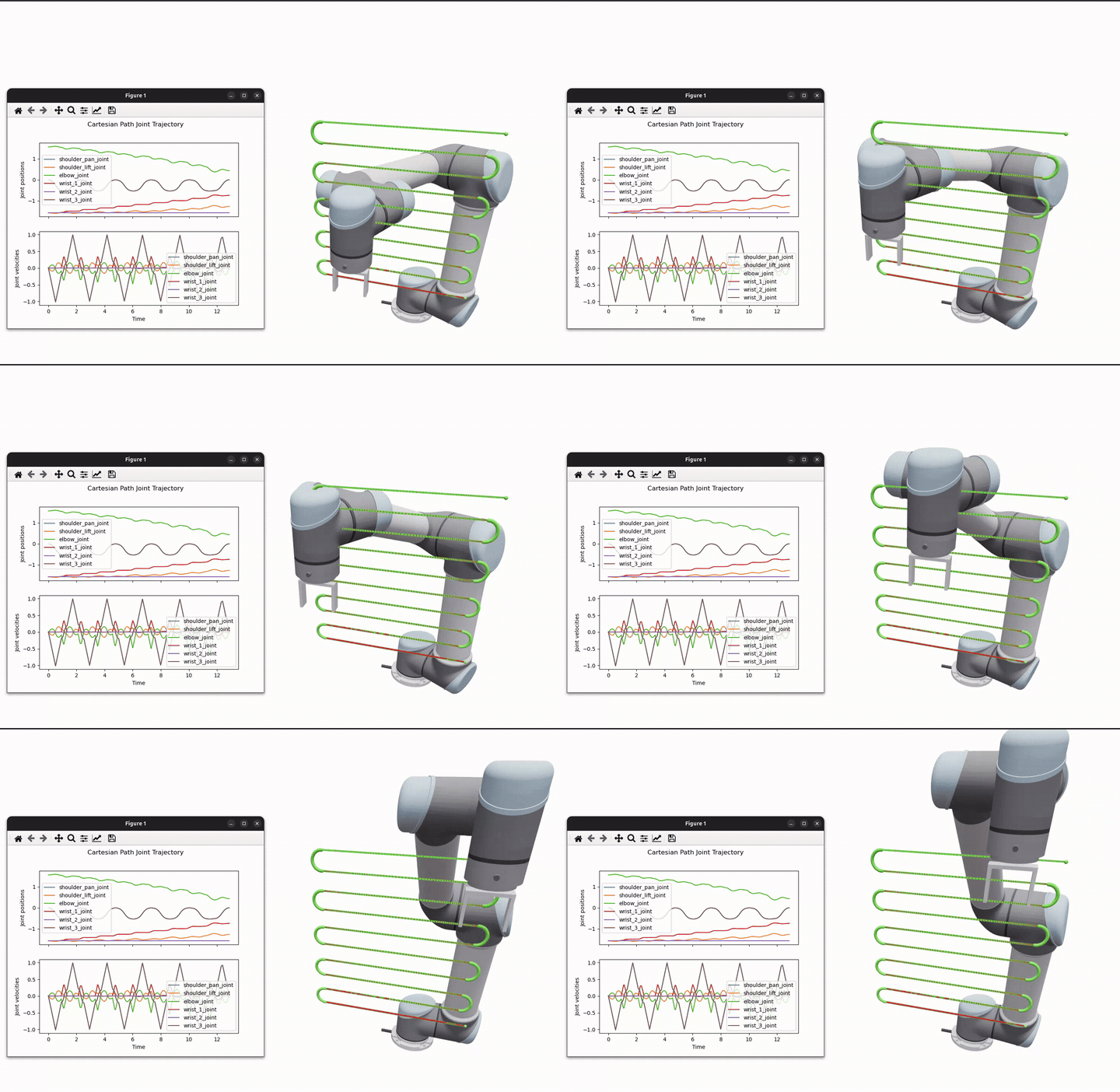
Cartesian path planning with a UR5 arm.
Approach
The planner builds an arc-length SE(3) reference from the waypoints (linear interpolation for position, SLERP for orientation). It then runs an offline servo loop using the OInK solver. At each control step, the planner advances the reference, solves one differential-IK step, and integrates the result. When the robot cannot keep up (e.g., near a singularity or joint velocity limit), the reference feedrate is throttled so that every committed sample stays within tolerance of the geometric path. If throttling fails after some number of iterations, the planner returns with a failure state.
Joint velocity and position limits are enforced inside the QP (and verified per step).
Two speed modes are exposed:
Bounded: the tool traces the path under a trapezoidal feedrate profile. The Cartesian tool speed ramps up to the commanded linear/angular maxima and back down to a stop at the path end, bounded by the commanded linear/angular acceleration maxima. The feedrate is throttled below that profile wherever the robot would otherwise leave the path tolerance or exceed its joint velocity limit. If the resulting motion still exceeds the joint velocity or acceleration limits (e.g. at a corner or near a singularity), the whole trace is re-timed slower and retried, so the commanded speeds and accelerations act as maxima, not fixed values. The result is a physically smooth motion rather than a constant-speed crawl.TimeOptimal: resolves the path to a dense joint path with the same Oink tracker, then time-parameterizes it with TOPP-RA over a straight-segment + circular-blend geometry. This way, the trajectory respects joint velocity and acceleration limits, and is time-optimal (the tool speed varies along the path).
Both modes return a JointTrajectory.
Quality metrics are computed on demand from that trajectory: computePeakLimitRatios returns the peak velocity/acceleration-to-limit ratios so the caller can see how close the result is to the joint limits, and computeAchievedPathLength returns the Cartesian distance traced by the tip frames.
Use Bounded for a predictable, velocity- and acceleration-limited Cartesian motion, and TimeOptimal when time-optimality matters.
Multiple end effectors
A CartesianPath may contain more than one end-effector frame.
The planner builds one tracking FrameTask per frame and advances all of them along a shared reference timeline, so the motions are traced simultaneously.
The throttling/tolerance logic uses the worst-case error across all frames, and computeAchievedPathLength sums the Cartesian distance across them.
Customizing the IK problem
By default the planner builds its own OInK solver.
This solver has one FrameTask per end-effector plus a nullspace ConfigurationTask.
It is bounded by VelocityLimit and PositionLimit constraints based on the robot joint limits.
For full control over the differential-IK problem, you can instead construct the planner with a CartesianPlannerComponents.
This lets you supply your own:
oink: the OInK solver instance.tracking_tasks: oneFrameTaskper end-effector, ordered to match the path’s tip frames.extra_tasks: additional tasks (e.g., a custom nullspace posture task).constraintsandbarriers: any constraints/control barrier functions to apply at every step.
The planner reuses these objects across all plan() calls and never mutates them apart from the tracking-task targets.
Any seed-dependent setup is the caller’s responsibility.
In this mode, the OInK-related fields of CartesianPlannerOptions (costs, gains, limits) are ignored.
However, the timing/tolerance fields (dt, speeds, max_*_error, speed_mode, scales) still apply.